In one sentence: Confidence intervals around a sample parameter (e.g., mean) express the range of values that are likely to include the true population parameter.
Step 1. Understand sampling and sample error.
Imagine we wanted to know the mean IQ of psychology undergrads. It would be pretty impossible for us to check the IQ of every single psychology undergrad in the world. Instead we would have to draw a sample. Based on our sample we will try to infer the mean intelligence of the psychology undergrad population. However, our conclusions will be different depending on the sample we draw – this is called sampling error. As long as we deal with samples instead of entire populations, there will always be an error.
Step 2. Confidence intervals
Confidence intervals characterise the uncertainty around a sample estimate. So, based on our example, instead of saying that we estimated that the mean IQ is 120, we would say that it is estimated that the mean IQ of the population of undergrad psychology student’s lies between 110 and 130. The confidence intervals tell us that our population mean lies within a specific interval. The said confidence can vary and it is pretty much up to us to choose. Most often people report 90 or 95 % confidence intervals. If we choose to calculate the 95% CI, then the CI will include the true population mean in 95 times out of a 100 cases.
Step 3. What affects the width of our confidence intervals?
The width of confidence intervals depends on two things:
CI for population mean can be easily calculated with the following formula
Confidence interval =
Now, what is t? – t is the value of the t-distribution that we need to look up in a t-distribution table. It is dependent on our choice of the confidence intervals (do we want 90%, 95% or maybe 99% confidence intervals) and the degrees of freedom. Looking at the formula, you should see that the bigger the t-value, the bigger will our confidence interval be. You multiply the t-value by the standard error and will get the margin of error. Now, all that’s left to do is to add and subtract the margin of error from our sample mean to get the confidence interval. Thankfully, we hardly ever will have to calculate CI by hand as SPSS does it nicely for us.
Step 5. Interpretation
The confidence level of for example 95% tells us that if we were to draw as many as 100 samples from the same population and calculate confidence intervals for each one, 95 of these confidence intervals would include the true population mean.
By Aleksandra Szafran (University of Dundee, Academic Year 2015-16)
Step 1. Understand sampling and sample error.
Imagine we wanted to know the mean IQ of psychology undergrads. It would be pretty impossible for us to check the IQ of every single psychology undergrad in the world. Instead we would have to draw a sample. Based on our sample we will try to infer the mean intelligence of the psychology undergrad population. However, our conclusions will be different depending on the sample we draw – this is called sampling error. As long as we deal with samples instead of entire populations, there will always be an error.
Step 2. Confidence intervals
Confidence intervals characterise the uncertainty around a sample estimate. So, based on our example, instead of saying that we estimated that the mean IQ is 120, we would say that it is estimated that the mean IQ of the population of undergrad psychology student’s lies between 110 and 130. The confidence intervals tell us that our population mean lies within a specific interval. The said confidence can vary and it is pretty much up to us to choose. Most often people report 90 or 95 % confidence intervals. If we choose to calculate the 95% CI, then the CI will include the true population mean in 95 times out of a 100 cases.
Step 3. What affects the width of our confidence intervals?
The width of confidence intervals depends on two things:
- Population Variation How much does the variable vary in the population? Do most students have similar scores around 120 or is the population more heterogeneous, i.e., many students have very low scores while others have very high scores. If the population has low variation, then any sample we choose will have low variation as well. If, however, the variation is large then it is possible that we draw a sample that results in wider confidence intervals.
- Sample Size: How big is the sample compared to the entire population? Is our sample just 10 or 1000 students out of 100000? If our sample is small, we really won’t have much information to accurately infer the population mean. Smaller samples would differ more from each other --> resulting in wider confidence intervals. Larger samples would probably not differ too much from each other --> smaller confidence intervals. The large sample reduces sampling error and causes us to have more faith in our mean estimate!
CI for population mean can be easily calculated with the following formula
Confidence interval =
Now, what is t? – t is the value of the t-distribution that we need to look up in a t-distribution table. It is dependent on our choice of the confidence intervals (do we want 90%, 95% or maybe 99% confidence intervals) and the degrees of freedom. Looking at the formula, you should see that the bigger the t-value, the bigger will our confidence interval be. You multiply the t-value by the standard error and will get the margin of error. Now, all that’s left to do is to add and subtract the margin of error from our sample mean to get the confidence interval. Thankfully, we hardly ever will have to calculate CI by hand as SPSS does it nicely for us.
Step 5. Interpretation
The confidence level of for example 95% tells us that if we were to draw as many as 100 samples from the same population and calculate confidence intervals for each one, 95 of these confidence intervals would include the true population mean.
By Aleksandra Szafran (University of Dundee, Academic Year 2015-16)
In one sentence: Beta coefficients in a regression tell us how much the predictor influences the dependent variable.
Step 1. What is a regression?
A regression allows us to predict an outcome variable from one or several predictor variables. For example, we could be interested in knowing what makes a comic book movie successful. We would judge the movie success by its box office earnings. There are many factors that could influence number of people going to see such a movie, for example: movie budget and the popularity of the main superhero (on a 1-10 scale). The regression could allow us to predict the box office success from movie’s budget and the superhero’s popularity if those two do contribute to the movie’s success.
Step 2. How to do a regression in SPSS?
 Now, let’s try to run a regression analysis in SPSS using our movie example.
Since we have two predictor variables, we need to run a multiple regression. The procedure is simple. Go to Analyze --> Regression --> Linear.
Now, let’s try to run a regression analysis in SPSS using our movie example.
Since we have two predictor variables, we need to run a multiple regression. The procedure is simple. Go to Analyze --> Regression --> Linear.
 Now, enter our variable of interest (box office earnings) as the dependent variable and our predictors as independent Variables. Press OK!
And that’s how we run a regression analysis.
Now, enter our variable of interest (box office earnings) as the dependent variable and our predictors as independent Variables. Press OK!
And that’s how we run a regression analysis.
Hurray! Now, let’s proceed to next step and look at our output.
Step 3. Regression equation
This is our output:
The output shows us that our model is statistically significant.
The regression equation is: Box Office Earnings = - 82.485 + (1.188 x Budget) + (74.187 x Super Hero Popularity) + Error
So, what does it all mean?
The fist number in green is our constant or intercept. It’s the value of y when all predictors are 0. In this case a movie is expected to lose 82.485 million if budget and SH popularity are both 0. The other two numbers (the red and blue ones) are the beta coefficients.
Step 4. Unstandardised and standardised beta coefficients.
The beta coefficients represent the slope of the regression line. It tells us the strength and direction of the relationship between predictors and outcome variable. The b values tell us how much each predictor contributes to our model.
In our case, both our beta values are positive and significant which means that as they increase the box office earnings as movie budget and superhero popularity increase. If the values were negative, we would naturally conclude a negative relationship. Moreover, the beta values tell us to what extent one predictor influences the outcome variable, if all other things are constant. In our example we can say that as superhero popularity increases by 1 unit, box office earnings (in million dollars) increase by 74.187 x 1. Similarly, as Budget is increased by 1 million the box office earnings will increase by 1.188 x 1 IF superhero popularity is held constant.
As you can see, our two beta coefficients are different: 74.187 and 1.188. You could be perhaps tempted to say that superhero popularity is a 62.45 times better predictor of movie earnings compared to movie budget ( 74.187/1.188 = 62.45). This is absolutely wrong!
As you should have noticed, in our regression equation we looked at unstandardised beta coefficients. What does it mean?
You should note that our units of measurement were very different. Superhero popularity scores ranged from 1 to 10. That’s a very small range, while movie budget which in real life is in millions, was expressed in hundreds ranging from 101.45 to 280.54. Much bigger numbers than 1-10. Those units of measurements affect the unstandardised beta coefficient.
But, if you look to the right of the output table, you will see the standardised beta coefficients. Those, in many ways are more useful and easier to interpret. They are called standardised as they are unaffected by the unit of measurements we use. So, in our example, whether we expressed movie budget in hundreds or millions, our standardised beta coefficients would be comparable. On the other hand, our unstandardised beta coefficients could not be easily compared to each other. Standardised beta coefficients are in standard deviations (SDs), i.e. as our predictor changes by one SD, by how many SDs does the outcome variable change?
In our example the standardised coefficients are as follows:
Movie budget = .250
Super hero popularity = .748
To understand this in more detail we need to know the SD of our outcome variable and predictors. For super hero popularity the SD is 2.47, for movie budget the SD is 51.45.
The SD for box office earnings is 244.68
Thus, the standardised beta value tells us that:
As movie budget increases by 51.45 (one SD), box office earnings increase by .250 x 244.68 = 61.17 As super hero popularity increases by 2.47 (one SD), box office earnings increase by 0.748 X 244.68 =183.02 Unlike in the case of unstandardised beta values, we can directly compare standardised ones. Therefore, in this case we can safely conclude that super hero popularity contributes more to a movie’s box office earnings compared to movie budget.
By Aleksandra Szafran (University of Dundee, Academic Year 2015-16)
Step 1. What is a regression?
A regression allows us to predict an outcome variable from one or several predictor variables. For example, we could be interested in knowing what makes a comic book movie successful. We would judge the movie success by its box office earnings. There are many factors that could influence number of people going to see such a movie, for example: movie budget and the popularity of the main superhero (on a 1-10 scale). The regression could allow us to predict the box office success from movie’s budget and the superhero’s popularity if those two do contribute to the movie’s success.
Step 2. How to do a regression in SPSS?
Now, let’s try to run a regression analysis in SPSS using our movie example.
Since we have two predictor variables, we need to run a multiple regression. The procedure is simple. Go to Analyze --> Regression --> Linear.
Now, enter our variable of interest (box office earnings) as the dependent variable and our predictors as independent Variables. Press OK!
And that’s how we run a regression analysis.Hurray! Now, let’s proceed to next step and look at our output.
Step 3. Regression equation
This is our output:
The output shows us that our model is statistically significant.
The regression equation is: Box Office Earnings = - 82.485 + (1.188 x Budget) + (74.187 x Super Hero Popularity) + Error
So, what does it all mean?
The fist number in green is our constant or intercept. It’s the value of y when all predictors are 0. In this case a movie is expected to lose 82.485 million if budget and SH popularity are both 0. The other two numbers (the red and blue ones) are the beta coefficients.
Step 4. Unstandardised and standardised beta coefficients.
The beta coefficients represent the slope of the regression line. It tells us the strength and direction of the relationship between predictors and outcome variable. The b values tell us how much each predictor contributes to our model.
In our case, both our beta values are positive and significant which means that as they increase the box office earnings as movie budget and superhero popularity increase. If the values were negative, we would naturally conclude a negative relationship. Moreover, the beta values tell us to what extent one predictor influences the outcome variable, if all other things are constant. In our example we can say that as superhero popularity increases by 1 unit, box office earnings (in million dollars) increase by 74.187 x 1. Similarly, as Budget is increased by 1 million the box office earnings will increase by 1.188 x 1 IF superhero popularity is held constant.
As you can see, our two beta coefficients are different: 74.187 and 1.188. You could be perhaps tempted to say that superhero popularity is a 62.45 times better predictor of movie earnings compared to movie budget ( 74.187/1.188 = 62.45). This is absolutely wrong!
As you should have noticed, in our regression equation we looked at unstandardised beta coefficients. What does it mean?
You should note that our units of measurement were very different. Superhero popularity scores ranged from 1 to 10. That’s a very small range, while movie budget which in real life is in millions, was expressed in hundreds ranging from 101.45 to 280.54. Much bigger numbers than 1-10. Those units of measurements affect the unstandardised beta coefficient.
But, if you look to the right of the output table, you will see the standardised beta coefficients. Those, in many ways are more useful and easier to interpret. They are called standardised as they are unaffected by the unit of measurements we use. So, in our example, whether we expressed movie budget in hundreds or millions, our standardised beta coefficients would be comparable. On the other hand, our unstandardised beta coefficients could not be easily compared to each other. Standardised beta coefficients are in standard deviations (SDs), i.e. as our predictor changes by one SD, by how many SDs does the outcome variable change?
In our example the standardised coefficients are as follows:
Movie budget = .250
Super hero popularity = .748
To understand this in more detail we need to know the SD of our outcome variable and predictors. For super hero popularity the SD is 2.47, for movie budget the SD is 51.45.
The SD for box office earnings is 244.68
Thus, the standardised beta value tells us that:
As movie budget increases by 51.45 (one SD), box office earnings increase by .250 x 244.68 = 61.17 As super hero popularity increases by 2.47 (one SD), box office earnings increase by 0.748 X 244.68 =183.02 Unlike in the case of unstandardised beta values, we can directly compare standardised ones. Therefore, in this case we can safely conclude that super hero popularity contributes more to a movie’s box office earnings compared to movie budget.
By Aleksandra Szafran (University of Dundee, Academic Year 2015-16)
What is it?
The Pearson’s correlation coefficient (also known as the Pearson’s product moment correlation coefficient) is a parametric test used to assess how two continuous variables co-relate in a linear manner. The standardised statistical output of the correlation coefficient is typically referred to as r, which specifies the strength and direction of the relationship between two variables (Steele et al., 2012).
Why use it?
The correlation coefficient is useful if we want to observe the relationship between two variables that already exists in a specific population. Through this observation, when one variable (x) changes we are able to see what happens to the second variable (y). More specifically, the correlation coefficient highlights four elements of a potential relationship (Field, 2014; Steele et al., 2014).
The benefit of r is that it can also tell us how much variance both variables share, i.e. how much of the variance in one variable is present in the second variable. This is achieved by calculating the coefficient of determination (R²), which is simply done by squaring r (Dancey & Reidy, 2014).
Checks & assumptions
As the Pearson’s correlation coefficient is a parametric test certain assumptions and checks must be made to ensure the data is fit for purpose. In total it is wise to undertake these seven checks before the test is run (Steele et al., 2012; Field, 2014):
 How to interpret the SPSS output
When it comes to interpreting the output of a Pearson’s correlation coefficient in SPSS there are several steps to be taken (Forshaw, 2007; Steele et al., 2012):
(1) The most important first step is to do a visual check of the scatterplot for signs that a correlation exists. If no apparent correlation is present, then it is likely there is no correlation. (2) Assuming you do observe a correlation pattern, then proceed to check the r value for the strength and direction of the relationship. (3) Once a correlation has been confirmed it is then necessary to ascertain whether it is in fact significant (p<0.05), or whether the correlation has arisen by chance (p>0.05). (4) At this point, if the level of significance is close to p=0.05 it is wise to check the impact of any outliers and how the result changes, if at all, when these are included or excluded.
Be aware
We can only correlate scores if they come from the same population, meaning we cannot compare relationships between different populations. Moreover, in a correlation we simply measure and observe relationships, we do not try to influence them or control them as we do in experiments, therefore we cannot state cause and effect from a correlation. It is also important to be aware of the ‘Third Variable Problem’, where changes in x and y may be due to the impact of an extraneous variable, which may or may not be under consideration (Field, 2014).
Worked example: The Daily Mile
Much has been made of the obesity rate in children and the need to improve children’s activity and fitness levels (BBC, 2015). A primary school in Dundee is interested in rolling out a scheme known as the ‘Daily Mile’ programme, where children run or walk a mile each day at school (The Scottish Government, 2015). Before the head teacher considers investing in the programme she is interested in finding out if a relationship exists between the weight of the children (variable w) and the time they take to complete a mile (variable t). She is aware the average weight for an 11 year old based on data from the WHO (Disabled World, 2016) is 36.25 kg (i.e., 35.6kg for girls, 36.9kg for boys), and the ‘healthy fitness zone’ pass rate to complete one mile at this age is 11 minutes 30 seconds (i.e. 12.00 mins for girls, 11.00 mins for boys) (Running School, 2007). One lunchtime she invites 40 pupils aged 11 years old (20 boys & 20 girls) to complete a mile and collects data about their weight and finish times (Table 1).
Assumptions & checks
The type of data collected is ratio data, for both the children’s weight and finish times, and was normally distributed, which means it can be used to run the Pearson’s correlation coefficient. By examining the scatterplot (Figure 9) we can see a positive linear relationship exists and data has been collected on both variables for all forty participants. Homoscedasticity is also present, with no disparity of variance along a potential line of best fit. Moreover, the head teacher was able to confirm that the assumption of independence of observation holds true. However, had it been the case that some children had agreed to run the mile together and finish together it would have violated this assumption. Also, there appear to be no outliers which might distort the r value.
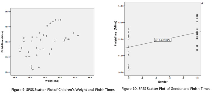 Moreover, as illustrated by Figure 10, there also appears to be a positive association between gender and finish times, with girls (coded as 1) taking longer to complete the mile than boys (coded as 0), which is in line with the estimates from the Running School (2007).
Interpretation
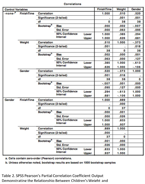
When Pearson’s correlation coefficient test was run in SPSS a significant, large, positive correlation existed between the children's weight and the time taken to complete one mile, r = .510, n=40, p<0.01. Higher weight levels in children were associated with longer times to complete the mile (Table 2). A significant, large, positive correlation was also found for the effect of gender on finish times, r = .520, n=40, p<0.01, with girls taking longer to complete the mile. However, a significant, medium, negative relationship was found between gender and weight, with girls weighing less than boys, r = -.373, n=40, p<0.05.
That said, the amount of variance shared by weight and finish times when gender was controlled for is .887, and significant (p<0.000). Therefore, the value of R² for the partial correlation is .79, meaning weight shares 79% of the variance in finish times, compared to 26% (.51 x .51) when gender was not controlled for. Whilst this association does not imply causality it does help to underscore the association between weight and fitness, which is the focus of efforts through programs such as the Daily Mile to reduce obesity.
By D. Anderson (University of Dundee, Academic Year 2015-16)
The Pearson’s correlation coefficient (also known as the Pearson’s product moment correlation coefficient) is a parametric test used to assess how two continuous variables co-relate in a linear manner. The standardised statistical output of the correlation coefficient is typically referred to as r, which specifies the strength and direction of the relationship between two variables (Steele et al., 2012).
Why use it?
The correlation coefficient is useful if we want to observe the relationship between two variables that already exists in a specific population. Through this observation, when one variable (x) changes we are able to see what happens to the second variable (y). More specifically, the correlation coefficient highlights four elements of a potential relationship (Field, 2014; Steele et al., 2014).
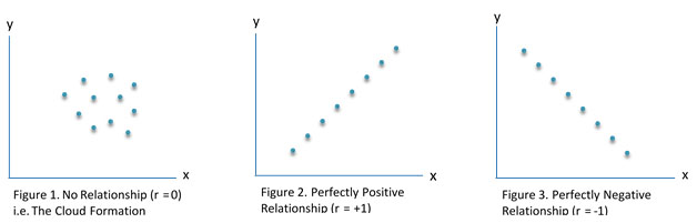
- If a relationship exists: The linear relationship between two variables is standardised into numerical form where it is represented by r (i.e. correlation coefficient), and lies on a continuum from -1 to +1. Where no linear relationship exists r = 0 (e.g. a change in x is not associated with a change in y) (Figure 1), however where a perfect positive linear relationship r = 1.0 or perfect negative linear relationship r = -1.0 exists (e.g., as x changes, y changes by the same amount).
- If the relationship is positive or negative: When a positive relationship exists an increase in x is associated with an increase in y (i.e. the value of r is greater than zero) (Figure 2), however when a negative relationship exists an increase in x is associated with a decrease in y (i.e. the value of r is less than zero) (Figure 3).
- The strength of the relationship: The magnitude of the relationship is demonstrated by the effect size. A small effect size occurs when r = 0.1, a medium effect size when r = 0.3, and a large effect size when r = 0.5 or more.
- The significance of the relationship: If r, as demonstrated by the p-value, is significantly different from zero then we can assume the identified relationship between the variables in our sample did not arise by chance (i.e., sampling error) and we have found a relationship of significance.
The benefit of r is that it can also tell us how much variance both variables share, i.e. how much of the variance in one variable is present in the second variable. This is achieved by calculating the coefficient of determination (R²), which is simply done by squaring r (Dancey & Reidy, 2014).
Checks & assumptions
As the Pearson’s correlation coefficient is a parametric test certain assumptions and checks must be made to ensure the data is fit for purpose. In total it is wise to undertake these seven checks before the test is run (Steele et al., 2012; Field, 2014):
- Data must be at the interval or ratio levels, or if one variable is interval or ratio then the other is dichotomous.
- Normally distributed data is required (i.e., not positively or negatively skewed).
- A linear relationship exists between the data (i.e., check via a scatter plot).
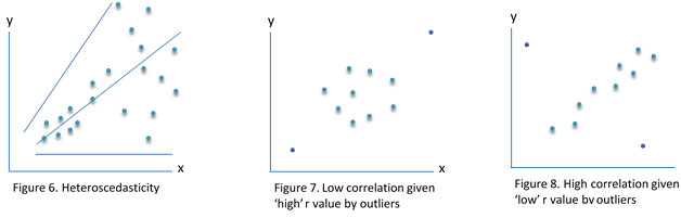
- Homoscedasticity is required with equal variance between variables (i.e., variances along the line of best fit are equally similar). This would be violated (i.e., heteroscedasticity) if for example, variances at one end of the scatter plot were of equal magnitude but at the opposite end the variances were widely dispersed, resulting in a funnel shape (Figure 6).
- Data is provided for each variable, both x and y.
- Independence of observation (i.e., participant scores are not influenced by other participants’ scores).
- Outliers are identified for potential distortion of the output, particularly in smaller sample sizes when one or two outlying scores can more easily impact the value of r. For example, a low correlation could be enhanced by some high outliers (Figure 7), whereas a high correlation could be limited by some low outliers (Figure 8) (Forshaw, 2007; Laerd Statistics, 2013).
How to interpret the SPSS outputWhen it comes to interpreting the output of a Pearson’s correlation coefficient in SPSS there are several steps to be taken (Forshaw, 2007; Steele et al., 2012):
(1) The most important first step is to do a visual check of the scatterplot for signs that a correlation exists. If no apparent correlation is present, then it is likely there is no correlation. (2) Assuming you do observe a correlation pattern, then proceed to check the r value for the strength and direction of the relationship. (3) Once a correlation has been confirmed it is then necessary to ascertain whether it is in fact significant (p<0.05), or whether the correlation has arisen by chance (p>0.05). (4) At this point, if the level of significance is close to p=0.05 it is wise to check the impact of any outliers and how the result changes, if at all, when these are included or excluded.
Be aware
We can only correlate scores if they come from the same population, meaning we cannot compare relationships between different populations. Moreover, in a correlation we simply measure and observe relationships, we do not try to influence them or control them as we do in experiments, therefore we cannot state cause and effect from a correlation. It is also important to be aware of the ‘Third Variable Problem’, where changes in x and y may be due to the impact of an extraneous variable, which may or may not be under consideration (Field, 2014).
Worked example: The Daily Mile
Much has been made of the obesity rate in children and the need to improve children’s activity and fitness levels (BBC, 2015). A primary school in Dundee is interested in rolling out a scheme known as the ‘Daily Mile’ programme, where children run or walk a mile each day at school (The Scottish Government, 2015). Before the head teacher considers investing in the programme she is interested in finding out if a relationship exists between the weight of the children (variable w) and the time they take to complete a mile (variable t). She is aware the average weight for an 11 year old based on data from the WHO (Disabled World, 2016) is 36.25 kg (i.e., 35.6kg for girls, 36.9kg for boys), and the ‘healthy fitness zone’ pass rate to complete one mile at this age is 11 minutes 30 seconds (i.e. 12.00 mins for girls, 11.00 mins for boys) (Running School, 2007). One lunchtime she invites 40 pupils aged 11 years old (20 boys & 20 girls) to complete a mile and collects data about their weight and finish times (Table 1).
| Pupil | Gender | Weight (kg) | Time to finish 1 mile (mins:secs) | Pupil | Gender | Weight (kg) | Time to finish 1 mile (mins:secs) |
|---|---|---|---|---|---|---|---|
| 1 | Boy | 35.5 | 11.45 | 21 | Girl | 33.7 | 11.35 |
| 2 | Boy | 35.9 | 11.45 | 22 | Girl | 34.6 | 13.15 |
| 3 | Boy | 36.2 | 12.17 | 23 | Girl | 34.9 | 10.59 |
| 4 | Boy | 36.2 | 10.39 | 24 | Girl | 35.2 | 12.15 |
| 5 | Boy | 36.4 | 12.55 | 25 | Girl | 35.2 | 10.15 |
| 6 | Boy | 36.4 | 12.11 | 26 | Girl | 35.8 | 10.32 |
| 7 | Boy | 36.9 | 10.31 | 27 | Girl | 36.2 | 12.03 |
| 8 | Boy | 37.2 | 12.49 | 28 | Girl | 36.3 | 13.31 |
| 9 | Boy | 37.3 | 12.55 | 29 | Girl | 36.9 | 10.31 |
| 10 | Boy | 37.8 | 11.42 | 30 | Girl | 36.9 | 11.01 |
| 11 | Boy | 38.6 | 12.19 | 31 | Girl | 37.3 | 11.59 |
| 12 | Boy | 38.9 | 14.11 | 32 | Girl | 37.4 | 14.12 |
| 13 | Boy | 39.3 | 12.33 | 33 | Girl | 37.8 | 11.45 |
| 14 | Boy | 39.4 | 13.29 | 34 | Girl | 38.2 | 12.28 |
| 15 | Boy | 40.5 | 14.03 | 35 | Girl | 38.3 | 13.05 |
| 16 | Boy | 40.6 | 11.45 | 36 | Girl | 39.1 | 13.04 |
| 17 | Boy | 40.8 | 14.15 | 37 | Girl | 39.4 | 13.15 |
| 18 | Boy | 41.1 | 13.59 | 38 | Girl | 39.8 | 13.42 |
| 19 | Boy | 41.2 | 14.42 | 39 | Girl | 40.1 | 12.45 |
| 20 | Boy | 14.02 | 40 | Girl | 38.7 | 13.23 |
The type of data collected is ratio data, for both the children’s weight and finish times, and was normally distributed, which means it can be used to run the Pearson’s correlation coefficient. By examining the scatterplot (Figure 9) we can see a positive linear relationship exists and data has been collected on both variables for all forty participants. Homoscedasticity is also present, with no disparity of variance along a potential line of best fit. Moreover, the head teacher was able to confirm that the assumption of independence of observation holds true. However, had it been the case that some children had agreed to run the mile together and finish together it would have violated this assumption. Also, there appear to be no outliers which might distort the r value.
Moreover, as illustrated by Figure 10, there also appears to be a positive association between gender and finish times, with girls (coded as 1) taking longer to complete the mile than boys (coded as 0), which is in line with the estimates from the Running School (2007).Interpretation
When Pearson’s correlation coefficient test was run in SPSS a significant, large, positive correlation existed between the children's weight and the time taken to complete one mile, r = .510, n=40, p<0.01. Higher weight levels in children were associated with longer times to complete the mile (Table 2). A significant, large, positive correlation was also found for the effect of gender on finish times, r = .520, n=40, p<0.01, with girls taking longer to complete the mile. However, a significant, medium, negative relationship was found between gender and weight, with girls weighing less than boys, r = -.373, n=40, p<0.05.
That said, the amount of variance shared by weight and finish times when gender was controlled for is .887, and significant (p<0.000). Therefore, the value of R² for the partial correlation is .79, meaning weight shares 79% of the variance in finish times, compared to 26% (.51 x .51) when gender was not controlled for. Whilst this association does not imply causality it does help to underscore the association between weight and fitness, which is the focus of efforts through programs such as the Daily Mile to reduce obesity.
By D. Anderson (University of Dundee, Academic Year 2015-16)
What is it?
The t-test is a parametric statistical test of normal distribution (to be more precisely a t-distribution) which allows us to compare two sample means of a continuous dependent variable, identify the amount by which they differ and determine whether this difference is statistically significant. The standardised statistical output is a t-value. Higher t-values are associated with lower p-values, which indicates the distribution of results are of statistical significance rather than a product of sampling error, when the null hypothesis is true (Field, 2014).
Why use a t-test?
The t-test is particularly useful in experiments where we want to assess the difference between two experimental conditions and there is one outcome variable (Keep in mind that there is also a One-Sample t-test where one sample mean is compared to a critical value to test whether it significantly differs from it or not.). In particular, its flexibility and sensitivity allows it to accommodate the nuances of experimental design when different participants (i.e., between-subjects design) partake in the two experimental conditions, or when the same participants are used in each condition (i.e., within-subject design). This means we can tailor the test to our selected experimental design (Steele, et al., 2012; Dancey & Reidy 2014):
The t-test is premised on a model which seeks to detect differences in the two sample group means in such a way as to apportion out systematic variance explained by the model (i.e., the experimental effect) and unsystematic variance which cannot be explained by the model (i.e., sampling error) (Field, 2014).
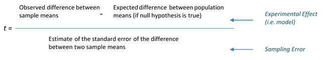
There are several important points to be mindful of when working with the top and bottom sections of the equation (Field, 2014):
In brief, the standard error is the standard deviation of the sample means drawn from the population. The standard error plays an important role within the t-test. Importantly, by dividing the average differences of means by the standard error this turns the t-test into a valuable tool of comparison, irrespective of the unit of measurement contained within the dependent variable. Moreover, it allows us to see the anticipated representativeness of the sample mean differences against the population. Large standard errors indicate a wide distribution of sample means, meaning there is a greater likelihood of large differences between samples. Whereas small sample errors indicate closely distributed means round the centred zero, meaning large differences would be unlikely (Field, 2014). In essence, when a small standard error is accompanied by a large difference between the sample means then we have a situation where the experimental manipulation has taken effect rather than an effect which has arisen by chance.
Be aware
Due to the potential increase in Type I error the t-test cannot be used if there are more than two groups for comparison, when for example the ANOVA test would be recommended. Moreover, as a parametric test, the assumptions of data at the interval/ratio level, normality of distribution, random sampling, assumption of independence and homogeneity of variance must be met (Steele, et al., 2014).
Taking the test with the daily mile
It is now eight weeks on from the initial assessment of the children’s times to complete the mile. During this time the children have completed the daily mile each day at school. The same children who took part in the initial trial mile at week zero have been tested again at the end of week eight. The head teacher now wishes to find out if there has been an overall improvement in finish times (irrespective of gender) and whether this has been significant or not.
A paired-samples t-test will allow us to compare the overall mean finish times between the two time trials. As highlighted by the SPSS output (Table 5), there has been a significant improvement in finish times from week zero to week eight, t(39) = 5.85, p=.000. Moreover, the standard error of the mean is small at 0.08, which indicates that the viability between different possible samples of 11-year-olds at the school would be small.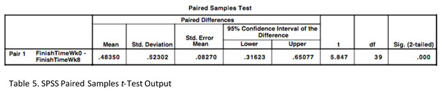 By D. Anderson (University of Dundee, Academic Year 2015-16)
The t-test is a parametric statistical test of normal distribution (to be more precisely a t-distribution) which allows us to compare two sample means of a continuous dependent variable, identify the amount by which they differ and determine whether this difference is statistically significant. The standardised statistical output is a t-value. Higher t-values are associated with lower p-values, which indicates the distribution of results are of statistical significance rather than a product of sampling error, when the null hypothesis is true (Field, 2014).
Why use a t-test?
The t-test is particularly useful in experiments where we want to assess the difference between two experimental conditions and there is one outcome variable (Keep in mind that there is also a One-Sample t-test where one sample mean is compared to a critical value to test whether it significantly differs from it or not.). In particular, its flexibility and sensitivity allows it to accommodate the nuances of experimental design when different participants (i.e., between-subjects design) partake in the two experimental conditions, or when the same participants are used in each condition (i.e., within-subject design). This means we can tailor the test to our selected experimental design (Steele, et al., 2012; Dancey & Reidy 2014):
- Independent t-test (Independent Measures): use when the two sets of mean scores come from two separate groups of participants.
- Paired Samples (Dependent Measures) t-test: use when the two sets of mean scores come from the same participants.
The t-test is premised on a model which seeks to detect differences in the two sample group means in such a way as to apportion out systematic variance explained by the model (i.e., the experimental effect) and unsystematic variance which cannot be explained by the model (i.e., sampling error) (Field, 2014).
There are several important points to be mindful of when working with the top and bottom sections of the equation (Field, 2014):
- If the experiment has no effect and the null hypothesis is true we would expect to see very little difference between the two sample means. Small differences might arise naturally, but large differences in means would be unexpected within one sample.
- Since no two samples are identical it is important to calculate the standard error which might have arisen between the two sample means in order that we can detect if the differences have arisen by chance or whether in fact we have a statistically meaningful result.
In brief, the standard error is the standard deviation of the sample means drawn from the population. The standard error plays an important role within the t-test. Importantly, by dividing the average differences of means by the standard error this turns the t-test into a valuable tool of comparison, irrespective of the unit of measurement contained within the dependent variable. Moreover, it allows us to see the anticipated representativeness of the sample mean differences against the population. Large standard errors indicate a wide distribution of sample means, meaning there is a greater likelihood of large differences between samples. Whereas small sample errors indicate closely distributed means round the centred zero, meaning large differences would be unlikely (Field, 2014). In essence, when a small standard error is accompanied by a large difference between the sample means then we have a situation where the experimental manipulation has taken effect rather than an effect which has arisen by chance.
Be aware
Due to the potential increase in Type I error the t-test cannot be used if there are more than two groups for comparison, when for example the ANOVA test would be recommended. Moreover, as a parametric test, the assumptions of data at the interval/ratio level, normality of distribution, random sampling, assumption of independence and homogeneity of variance must be met (Steele, et al., 2014).
Taking the test with the daily mile
It is now eight weeks on from the initial assessment of the children’s times to complete the mile. During this time the children have completed the daily mile each day at school. The same children who took part in the initial trial mile at week zero have been tested again at the end of week eight. The head teacher now wishes to find out if there has been an overall improvement in finish times (irrespective of gender) and whether this has been significant or not.
A paired-samples t-test will allow us to compare the overall mean finish times between the two time trials. As highlighted by the SPSS output (Table 5), there has been a significant improvement in finish times from week zero to week eight, t(39) = 5.85, p=.000. Moreover, the standard error of the mean is small at 0.08, which indicates that the viability between different possible samples of 11-year-olds at the school would be small.
By D. Anderson (University of Dundee, Academic Year 2015-16)To understand what a co-variate is, it is first helpful to understand the purpose of an ANOVA (analysis of variance).
ANOVA
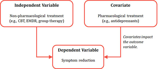
A one-way ANOVA is used where a researcher wants to compare the means of more than two conditions; typically, three or more mean scores are compared. ANOVA can inform as to whether there are significant differences between the means of the groups you want to compare. For example, a researcher may be interested in investigating non-pharmacological treatment for post-traumatic stress disorder and outcome (e.g., whether symptoms decrease). There may be three levels of the independent variable (treatment), for example, (1) cognitive behavioural therapy, (2) eye movement desensitization and reprocessing therapy and (3) group therapy. Symptom reduction is the only dependent variable. The one-way ANOVA would look to compare the treatment groups to see if there were any significant differences in mean scores between them. There are, however, other variables that may be correlated with the outcome variable of symptom reduction; for example, whether individuals with depression are receiving pharmacological interventions such as antidepressants, or the level of social support the individual has. These ‘additional’ variables can be entered as covariates. An ANCOVA (analysis of covariance) or MANCOVA (multivariate analysis of covariance) will include and statistically control for the influence these covariates may be having on the dependent variable. An ANCOVA is therefore an extension of the one-way ANOVA, in that it includes covariates. A MANCOVA is an extension of an ANCOVA because it encompasses more than one dependent variable, as well as also including covariates.
There are two main reasons why is it is useful to include covariates in an ANOVA analysis:
Assumptions of an ANCOVA
Before an ANCOVA can be conducted, there are several assumptions that the data need to meet:
ANOVA
A one-way ANOVA is used where a researcher wants to compare the means of more than two conditions; typically, three or more mean scores are compared. ANOVA can inform as to whether there are significant differences between the means of the groups you want to compare. For example, a researcher may be interested in investigating non-pharmacological treatment for post-traumatic stress disorder and outcome (e.g., whether symptoms decrease). There may be three levels of the independent variable (treatment), for example, (1) cognitive behavioural therapy, (2) eye movement desensitization and reprocessing therapy and (3) group therapy. Symptom reduction is the only dependent variable. The one-way ANOVA would look to compare the treatment groups to see if there were any significant differences in mean scores between them. There are, however, other variables that may be correlated with the outcome variable of symptom reduction; for example, whether individuals with depression are receiving pharmacological interventions such as antidepressants, or the level of social support the individual has. These ‘additional’ variables can be entered as covariates. An ANCOVA (analysis of covariance) or MANCOVA (multivariate analysis of covariance) will include and statistically control for the influence these covariates may be having on the dependent variable. An ANCOVA is therefore an extension of the one-way ANOVA, in that it includes covariates. A MANCOVA is an extension of an ANCOVA because it encompasses more than one dependent variable, as well as also including covariates.
Figure 1: Conceptual diagram of ANCOVA
There are two main reasons why is it is useful to include covariates in an ANOVA analysis:
- In an ANOVA analysis, it is possible to explain the effect that the experiment has had by comparing variability: the amount that can be attributed to the experiment and the amount that is unaccounted for by the experiment and is therefore ‘unexplained’ variance. Covariates may be able to explain some of this unexplained variance when they are included in the covariance analysis and thus explain some of the error variance. Consequently, the effect of the independent variables is clearer.
- Including and controlling for covariates in the analysis quantifies their influence on the dependent variable.
Assumptions of an ANCOVA
Before an ANCOVA can be conducted, there are several assumptions that the data need to meet:
- Both the covariate and dependent variable must be continuous variables (interval or ratio level)
- The independent variable should consist of two or more levels (e.g. gender: male and female)
- Each participant must be in a different experimental group and participants should not be in more than one group (otherwise known as independence of observations)
- Outliers in the data must not exist
- The dependent variable should be normally distributed, e.g., assessed by Shapiro-Wilk test of normality.
- There must be homogeneity of variances (the assumption that all groups have identical or similar variances). This can be assessed using Levene’s test.
- The covariate should be linearly related to your dependent variable at each level of the independent variable in order to reduce error variance and so increase ANCOVA sensitivity.
- Homoscedasticity must exist (where the error variance is equivalent across all values of the independent variables).
- There must not be any interaction between the covariate and independent variable (otherwise known as homogeneity of regression slopes).
Sphericity is one of the assumptions that should be met for a repeated-measures ANOVA. This assumption requires variances of the differences between experimental conditions to be approximately equal. To illustrate this:
Case study
A researcher wanted to investigate peak expiratory flow, measured in litres per minute (l/min), in seven non-smoking men aged 50 at three different times: firstly after smoking a cigarette, secondly after exercising for 30 minutes and thirdly in normal circumstances (control condition).
The differences between experimental conditions (here: time points) are calculated and then the variance of the difference scores are derived as -25, -98 and -63, respectively. Prima facie, it appears that these variance differences are very varied and not at all equal; it could therefore be assumed that the assumption of sphericity had been violated. However, to statistically assess this hypothesis, Mauchly’s Test of Sphericity is used in SPSS to test the null hypothesis that the variance of differences between conditions are equal. If Mauchly’s test is significant (p < .05), then significant differences between the variances of differences between conditions exist and the assumption of sphericity has been violated. In this scenario, the researcher should not hold much confidence in the F statistic SPSS calculates and should be aware that the likelihood of Type 2 error is increased. In this case, SPSS offers different corrections of the degrees of freedom (e.g., Greenhouse-Geisser correction of Huynh-Feldt correction) leading to a trustworthy F statistic. If Mauchly’s test is insignificant (p > .05), then it is possible to conclude that the variances of differences between conditions are approximately equal and the assumption of sphericity has been met. Providing that other assumptions are met for a repeated measures ANOVA, it may then be used.
By Kathryn Wilson (University of Dundee, Academic Year 2015-16)
Case study
A researcher wanted to investigate peak expiratory flow, measured in litres per minute (l/min), in seven non-smoking men aged 50 at three different times: firstly after smoking a cigarette, secondly after exercising for 30 minutes and thirdly in normal circumstances (control condition).
| Participant | Time 1: After smoking | Time 2: After exercise | Time 3: Control condition | Time 1-Time 2 | Time 1–Time 3 | Time 2–Time 3 |
|---|---|---|---|---|---|---|
| 1 | 575 | 570 | 590 | 5 | -15 | -20 |
| 2 | 590 | 600 | 610 | -10 | -20 | -10 |
| 3 | 590 | 600 | 600 | -10 | -20 | 0 |
| 4 | 585 | 585 | 590 | 0 | -5 | -5 |
| 5 | 570 | 575 | 588 | -5 | -18 | -13 |
| 6 | 585 | 590 | 600 | -5 | -15 | -10 |
| 7 | 575 | 575 | 580 | 0 | -5 | -5 |
| Variance: | -25 | -98 | -63 |
By Kathryn Wilson (University of Dundee, Academic Year 2015-16)
When conducting research in the real world it is unlikely that we would encounter a scenario where one variable exclusively predicts the outcome in another, since most variables will be highly interrelated with others. Moderation and mediation are two of the ways that variables can relate to each other which we need to take into account when analysing our results.
Moderation
Moderation occurs when two predictor variables have a combined effect on an outcome variable (i.e. one variable has a relationship with the outcome variable, but this relationship changes depending on the values of another variable, the moderator), this may also be referred to as an interaction effect.
We can visualise how the moderator affects the relationship between the predictor variable and the outcome variable as follows: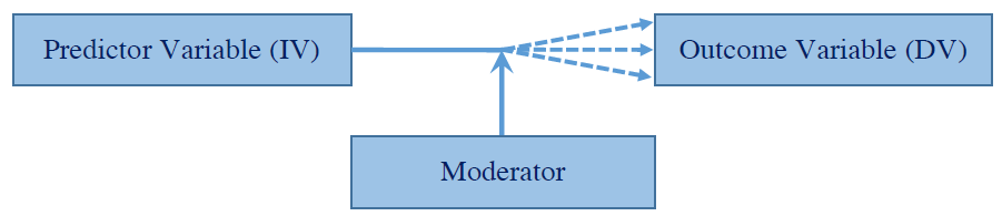 As the figure above demonstrates, the moderator affects the relationship that the predictor
variable has with the outcome variable. The relationship between the predictor and outcome may increase, decrease or stay the same depending on different levels of the moderator. As an example of how this might work, let’s say that we were investigating whether working long hours leads to decreased relationship satisfaction with a partner. If we conducted a simple regression it may appear that working long hours does lead to decreased relationship satisfaction.
As the figure above demonstrates, the moderator affects the relationship that the predictor
variable has with the outcome variable. The relationship between the predictor and outcome may increase, decrease or stay the same depending on different levels of the moderator. As an example of how this might work, let’s say that we were investigating whether working long hours leads to decreased relationship satisfaction with a partner. If we conducted a simple regression it may appear that working long hours does lead to decreased relationship satisfaction.
However, there may be a third variable which moderates the effect of working long hours on relationship satisfaction, such as, strength of relationship. If this variable is included in our analysis it may influence the way that working long hours impacts on relationship satisfaction. So, we may see a moderation (or interaction) like the one depicted below: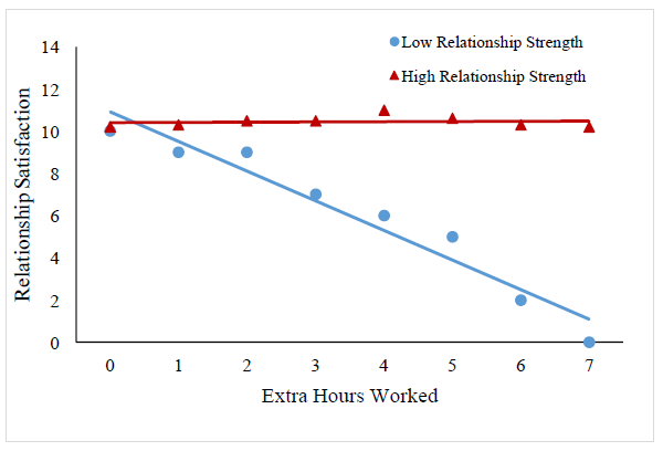 In the example above, working long hours only affects relationship satisfaction in low-strength relationships. In high-strength relationships, working long hours appears to have no effect on relationship satisfaction. ‘strength of relationship’ therefore moderates the impact that working long hours has on relationship satisfaction.
Mediation
Unlike moderators, which can affect the strength or direction of the relationship between a predictor and an outcome; mediators can be said to better explain the relationship between the predictor and the outcome. We can visualise the relationship between the predictor variable, the mediator, and the outcome variable using an example as follows: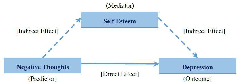 In this scenario we may already be aware that there is a significant relationship between having negative thoughts and depression (having more negative thoughts leads to scoring higher on a depression inventory). However, we may be interested in whether negative thoughts affect self esteem and whether this effect on self esteem would better explain (mediate) the relationship between negative thoughts and depression.
Testing for Mediation
In order to test for mediation we firstly need to use simple regression to examine several relationships:
Summary
Moderators - Affect the strength and/or direction of the relationship between two variables. Mediators - Provide a more specific explanation of why a relationship exists between two variables.
By Martin Bell (University of Dundee, Academic Year 2016-17)
Moderation
Moderation occurs when two predictor variables have a combined effect on an outcome variable (i.e. one variable has a relationship with the outcome variable, but this relationship changes depending on the values of another variable, the moderator), this may also be referred to as an interaction effect.
We can visualise how the moderator affects the relationship between the predictor variable and the outcome variable as follows:
As the figure above demonstrates, the moderator affects the relationship that the predictor
variable has with the outcome variable. The relationship between the predictor and outcome may increase, decrease or stay the same depending on different levels of the moderator. As an example of how this might work, let’s say that we were investigating whether working long hours leads to decreased relationship satisfaction with a partner. If we conducted a simple regression it may appear that working long hours does lead to decreased relationship satisfaction.However, there may be a third variable which moderates the effect of working long hours on relationship satisfaction, such as, strength of relationship. If this variable is included in our analysis it may influence the way that working long hours impacts on relationship satisfaction. So, we may see a moderation (or interaction) like the one depicted below:
In the example above, working long hours only affects relationship satisfaction in low-strength relationships. In high-strength relationships, working long hours appears to have no effect on relationship satisfaction. ‘strength of relationship’ therefore moderates the impact that working long hours has on relationship satisfaction.Mediation
Unlike moderators, which can affect the strength or direction of the relationship between a predictor and an outcome; mediators can be said to better explain the relationship between the predictor and the outcome. We can visualise the relationship between the predictor variable, the mediator, and the outcome variable using an example as follows:
In this scenario we may already be aware that there is a significant relationship between having negative thoughts and depression (having more negative thoughts leads to scoring higher on a depression inventory). However, we may be interested in whether negative thoughts affect self esteem and whether this effect on self esteem would better explain (mediate) the relationship between negative thoughts and depression.Testing for Mediation
In order to test for mediation we firstly need to use simple regression to examine several relationships:
- The relationship between the predictor (negative thoughts) and the outcome (depression)
- The relationship between the predictor (negative thoughts) and the mediator (self esteem)
- The relationship between the mediator (self esteem) and the outcome (depression)
Summary
Moderators - Affect the strength and/or direction of the relationship between two variables. Mediators - Provide a more specific explanation of why a relationship exists between two variables.
By Martin Bell (University of Dundee, Academic Year 2016-17)
Sample versus population
Let’s suppose we are interested in finding the mean number of books people in Scotland aged between twenty and thirty read per year. It would be pretty impossible to ask every single person in Scotland aged between twenty and thirty how many books they read in the past year. We therefore collect data from a sample of participants. We use the parameters of this sample to make inferences about the parameters of the population. In so doing, there will always be a certain amount of error in our estimate.
The standard error of the mean is a measure of how close a sample mean is likely to be to the true population mean.
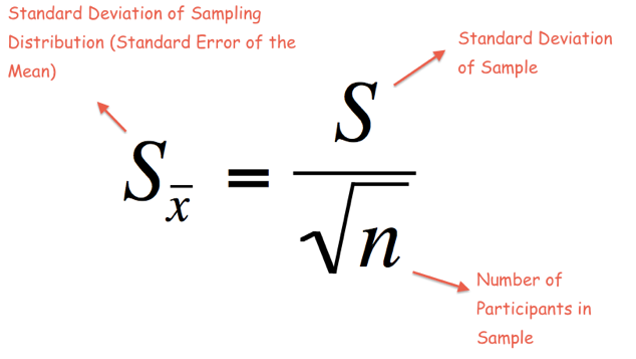
The standard error of the mean
In our data file, we have a total of 50 samples each of which consists of 20 participants. For each sample, we have a sample mean. So we have 50 sample means. The standard error of the mean is the standard deviation of the distribution of these sample means. The mean of all the sample means, as the number of samples becomes very large, is the population mean.
Here is the bell-curved sampling distribution of all the means: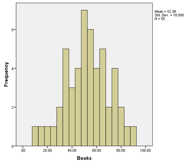 The formula to calculate the standard error of the mean is the following:
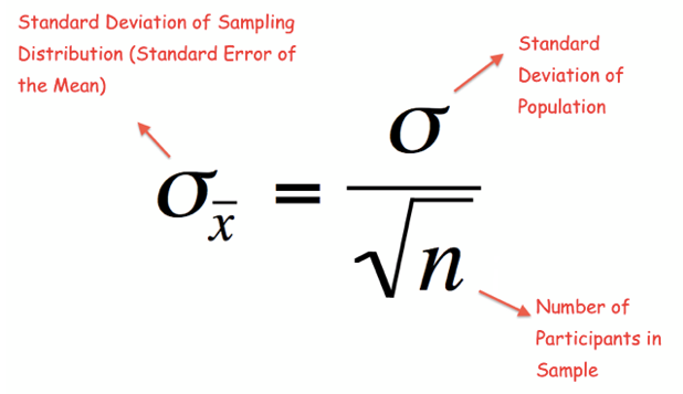 In order to use this formula, we would need to know the standard deviation of the population. However, in most cases we do not know the standard deviation of the population. Then, we use the standard deviation of the sample as an approximation for the standard deviation of the population. That is, we use the formula below:
 Let’s assume the mean of one of our samples is 47 and the standard deviation is 18. The number of participants is 20. Therefore, the standard error of the mean in this sample is:
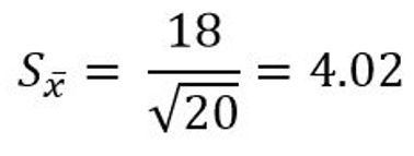 As we can see, the sample size is in the denominator and therefore a larger sample yields a smaller error. This is important because it means that with a larger sample size we can better estimate the population mean. In other words, the sample mean is a better, but not perfect, representation of the population mean.
By Jessica Schulz (University of Dundee, Academic Year 2016-17)
Let’s suppose we are interested in finding the mean number of books people in Scotland aged between twenty and thirty read per year. It would be pretty impossible to ask every single person in Scotland aged between twenty and thirty how many books they read in the past year. We therefore collect data from a sample of participants. We use the parameters of this sample to make inferences about the parameters of the population. In so doing, there will always be a certain amount of error in our estimate.
The standard error of the mean is a measure of how close a sample mean is likely to be to the true population mean.
The standard error of the mean
In our data file, we have a total of 50 samples each of which consists of 20 participants. For each sample, we have a sample mean. So we have 50 sample means. The standard error of the mean is the standard deviation of the distribution of these sample means. The mean of all the sample means, as the number of samples becomes very large, is the population mean.
Here is the bell-curved sampling distribution of all the means:
The formula to calculate the standard error of the mean is the following:
In order to use this formula, we would need to know the standard deviation of the population. However, in most cases we do not know the standard deviation of the population. Then, we use the standard deviation of the sample as an approximation for the standard deviation of the population. That is, we use the formula below:
Let’s assume the mean of one of our samples is 47 and the standard deviation is 18. The number of participants is 20. Therefore, the standard error of the mean in this sample is:
As we can see, the sample size is in the denominator and therefore a larger sample yields a smaller error. This is important because it means that with a larger sample size we can better estimate the population mean. In other words, the sample mean is a better, but not perfect, representation of the population mean.By Jessica Schulz (University of Dundee, Academic Year 2016-17)
Abstract
A partial correlation measures the relationship between two variables while controlling for the effect that a third variable has on them both, while a semi-partial correlation measures the relationship between two variables while controlling for the effect of a third variable on only one of the two.
What Is A Correlation?
Correlation is a relationship between two variables. It measures the extent to which two variables are related. When measuring the linear relationship between two continuous variables we normally use Pearson’s correlation coefficient r. We do not use covariance because it depends upon the units of measure. By dividing covariance with standard deviations of the variables, we get standardised version of the covariance which is basically the correlation coefficient.
However, if we square our correlation coefficient we get the coefficient of determination R^2, which tells us the proportion of variance both variables share with each other.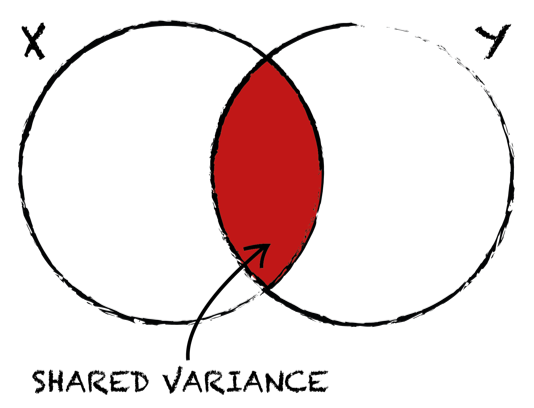 Therefore, whenever we want to compare one correlation to the other or talk about the amount of shared variance between two variables, we must always square our correlation coefficient.
Example
Let’s say we are interested in the relationship between academic performance and socioeconomic status. We have a dataset with N participants and we collected information about their socioeconomic status (X), their academic performance (Y) and their intelligence (Z) and measured the correlations between all three variables.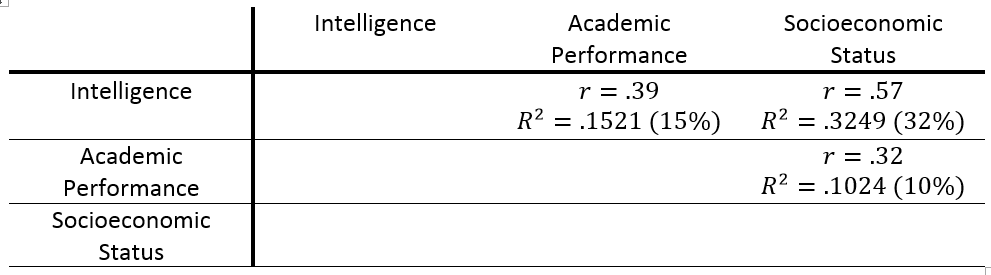 For the sake of illustration let’s say that all our relationships are statistically significant (p < .05). Our correlation coefficient tells us that as socioeconomic status increases, so does academic performance (rXY = .32). It also tells us that as intelligence increases, academic performance increases (rZY = .39) and so does socioeconomic status (rZX = 572). Taking a step further, we can look at coefficients of determination R^2, which tell us that socioeconomic status accounts for 10% of the variability in academic performance, whilst intelligence accounts for 15% of the variability in academic performance and 32% of the variance in socioeconomic status. Because intelligence accounts for almost one third of the variance in academic performance, we can suspect that some of the variance in academic performance explained by socioeconomic status is not unique and could be accounted for by intelligence.
To measure the pure relationship between academic performance and socioeconomic status we will have to hold the effect of intelligence constant by running a partial correlation.
Partial Correlation
With partial correlation, we measure the relationship between two variables while controlling for the effects of a third variable on the two variables in the original correlation.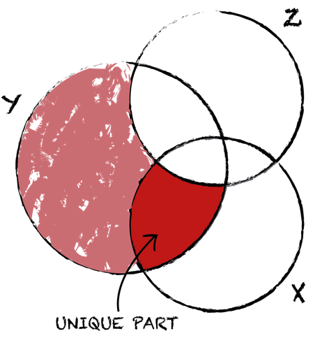 In partial correlation, we first calculate the relationship between Y and Z and partial out the overlap. Second, we calculate the relationship between X and Z and exclude the overlap. We control for Z in both variables, thus taking away any parts that Z explains in Y and in X. What we then look at is the unique part of X alone and how this relates to what is left of Y.
Example
In our case, we want to control for intelligence in both socioeconomic status and academic performance. Therefore, we look at the unique part that is due to socioeconomic status alone and how it relates to what is left of academic performance without the overlap from intelligence.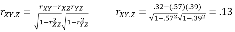 Let’s assume that this correlation is still significant (p < .05). We can notice that after controlling for the effect of intelligence, the partial correlation between academic performance and socioeconomic status (rXY.Z = .13) is considerably lower than before (rXY = .32). The amount of shared variance has dramatically decreased from 10% when intelligence was not controlled for, to only 2% (R^2 = .02). Running partial correlation has shown us that socioeconomic status alone only explains 2% of variation in academic performance.
With partial correlation, we measure the relationship between X and Y while holding Z constant for both X and Y. Sometimes we want to hold Z constant for only one of the other two variables. When that is the case, we are dealing with a semi-partial correlation.
Semi-Partial Correlation
Semi-partial correlation is most often used when we want to show that some variable contributes to the variance above and beyond the other variable. We measure the relationship between two variables while controlling for the effects of a third variable on only of the two variables in the original correlation.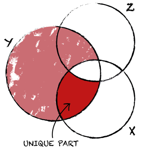 In semi-partial correlation, we calculate the relationship between X and Z and take out the overlap between X and Z, but not between Y and Z. We control for Z only in variable X, thus ignoring the part where Z overlaps with Y. We again look at the same unique part of X alone and how it relates to the whole of Y, including the overlap with Z.
Example
So, in our case we want to control only for the effect of intelligence on socioeconomic status, while the effect of intelligence on academic performance is ignored. Therefore, we look at the unique part that is due to socioeconomic status alone and how it relates to the whole of academic performance, including any variance shared with intelligence.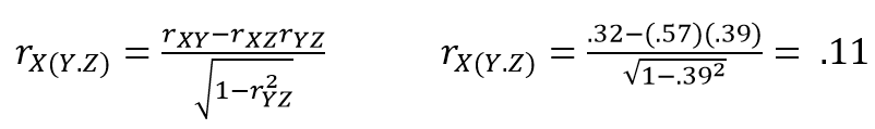 Under the assumption that this correlation is still significant (p < .05), we noticed that after controlling for the effect of intelligence on only socioeconomic status but not on academic performance, we ended up with even lower semi-partial correlation between academic performance and socioeconomic status (rX(Y.Z) = .13). After squaring the correlation coefficient, we are left with R^2 of .01, telling us that the amount of shared variance has even further decreased to only 1%.
The Main Difference
When measuring partial and semi-partial correlation, the unique part of our variable which we relate to the parts of other variables always stays the same. The main difference is to what parts of the other variables the unique part of our variable relates to and how big the other parts are. Since the unique part in semi-partial correlation relates to a larger bit, the semi-partial correlation will always be smaller than partial correlation.
By Petra Lipnik (University of Dundee, Academic Year 2016-17)
A partial correlation measures the relationship between two variables while controlling for the effect that a third variable has on them both, while a semi-partial correlation measures the relationship between two variables while controlling for the effect of a third variable on only one of the two.
What Is A Correlation?
Correlation is a relationship between two variables. It measures the extent to which two variables are related. When measuring the linear relationship between two continuous variables we normally use Pearson’s correlation coefficient r.
We do not use covariance because it depends upon the units of measure. By dividing covariance with standard deviations of the variables, we get standardised version of the covariance which is basically the correlation coefficient.However, if we square our correlation coefficient we get the coefficient of determination R^2, which tells us the proportion of variance both variables share with each other.
Therefore, whenever we want to compare one correlation to the other or talk about the amount of shared variance between two variables, we must always square our correlation coefficient.Example
Let’s say we are interested in the relationship between academic performance and socioeconomic status. We have a dataset with N participants and we collected information about their socioeconomic status (X), their academic performance (Y) and their intelligence (Z) and measured the correlations between all three variables.
For the sake of illustration let’s say that all our relationships are statistically significant (p < .05). Our correlation coefficient tells us that as socioeconomic status increases, so does academic performance (rXY = .32). It also tells us that as intelligence increases, academic performance increases (rZY = .39) and so does socioeconomic status (rZX = 572). Taking a step further, we can look at coefficients of determination R^2, which tell us that socioeconomic status accounts for 10% of the variability in academic performance, whilst intelligence accounts for 15% of the variability in academic performance and 32% of the variance in socioeconomic status. Because intelligence accounts for almost one third of the variance in academic performance, we can suspect that some of the variance in academic performance explained by socioeconomic status is not unique and could be accounted for by intelligence.To measure the pure relationship between academic performance and socioeconomic status we will have to hold the effect of intelligence constant by running a partial correlation.
Partial Correlation
With partial correlation, we measure the relationship between two variables while controlling for the effects of a third variable on the two variables in the original correlation.
In partial correlation, we first calculate the relationship between Y and Z and partial out the overlap. Second, we calculate the relationship between X and Z and exclude the overlap. We control for Z in both variables, thus taking away any parts that Z explains in Y and in X. What we then look at is the unique part of X alone and how this relates to what is left of Y.Example
In our case, we want to control for intelligence in both socioeconomic status and academic performance. Therefore, we look at the unique part that is due to socioeconomic status alone and how it relates to what is left of academic performance without the overlap from intelligence.
Let’s assume that this correlation is still significant (p < .05). We can notice that after controlling for the effect of intelligence, the partial correlation between academic performance and socioeconomic status (rXY.Z = .13) is considerably lower than before (rXY = .32). The amount of shared variance has dramatically decreased from 10% when intelligence was not controlled for, to only 2% (R^2 = .02). Running partial correlation has shown us that socioeconomic status alone only explains 2% of variation in academic performance.With partial correlation, we measure the relationship between X and Y while holding Z constant for both X and Y. Sometimes we want to hold Z constant for only one of the other two variables. When that is the case, we are dealing with a semi-partial correlation.
Semi-Partial Correlation
Semi-partial correlation is most often used when we want to show that some variable contributes to the variance above and beyond the other variable. We measure the relationship between two variables while controlling for the effects of a third variable on only of the two variables in the original correlation.
In semi-partial correlation, we calculate the relationship between X and Z and take out the overlap between X and Z, but not between Y and Z. We control for Z only in variable X, thus ignoring the part where Z overlaps with Y. We again look at the same unique part of X alone and how it relates to the whole of Y, including the overlap with Z.Example
So, in our case we want to control only for the effect of intelligence on socioeconomic status, while the effect of intelligence on academic performance is ignored. Therefore, we look at the unique part that is due to socioeconomic status alone and how it relates to the whole of academic performance, including any variance shared with intelligence.
Under the assumption that this correlation is still significant (p < .05), we noticed that after controlling for the effect of intelligence on only socioeconomic status but not on academic performance, we ended up with even lower semi-partial correlation between academic performance and socioeconomic status (rX(Y.Z) = .13). After squaring the correlation coefficient, we are left with R^2 of .01, telling us that the amount of shared variance has even further decreased to only 1%.The Main Difference
When measuring partial and semi-partial correlation, the unique part of our variable which we relate to the parts of other variables always stays the same. The main difference is to what parts of the other variables the unique part of our variable relates to and how big the other parts are. Since the unique part in semi-partial correlation relates to a larger bit, the semi-partial correlation will always be smaller than partial correlation.
By Petra Lipnik (University of Dundee, Academic Year 2016-17)
Abstract
Hierarchical multiple regression is one of the methods of adding predictors into the multiple regression model where experimenter decides the order in which variables are entered into the model.
What Is A Multiple Regression?
Multiple regression is a natural extension of simple linear regression and is used when we want to predict outcome from multiple predictors. The general purpose of multiple regression is to learn more about the relationship between several independent variables or predictors and a dependent variable or an outcome. It is a hypothetical model of the relationship between several variables.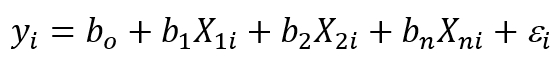 Adding Predictors
Does the order in which we enter predictors matter?
In theory, it shouldn’t as the regression equation is of additive nature. In practice, however, all predictors correlate with each other to some extent and it is nearly impossible to find two predictors that are completely unrelated to each other. As soon as predictors are correlated there is a change in beta weight whenever a new predictor is added to the equation. Therefore, the answer is yes, the order does matter whenever the predictors are correlated.
Different methods of adding predictors to the regression model are:
In hierarchical multiple regression, we add the known predictors into the regression model first, with new predictors entered in separate blocks. The predictor is chosen to be added in the first block based on a theory or previous research that has shown that it is the main driving predictor to predict our outcome. The new predictors that we are interested in are then added in separate blocks. This way we can see the contribution of the new predictor when all other predictors are held constant.
When running hierarchical multiple regression we look at two things:
R^2 change, which tells us whether adding new predictors to our model improves our model significantly.
Beta weights of all our predictors, because we want to see how good our predictors are.
Remember! Hierarchical multiple regression relies on the researchers to know what they are doing as they make all the decisions.
When Would You Use It
We use hierarchical regression when we want to see whether predictors of our interest explain statistically significant amount of variance in our outcome after controlling for all other predictors. For example, we would use it when testing a new theory, as it tells us if in addition to this main predictor that we have, are there any other predictors that may contribute to the model above and beyond the one that is already there.
Example
Let’s assume that students studying abroad in UK filled out a questionnaire where they were asked to rate their Stress from Studying, Stress from Living Away from their Families, Stress from Financial Issues and their Satisfaction with Life. Let’s say that previous studies have shown that the Stress from Studying is the most important predictor for Life Satisfaction and we would like to know whether Stress from Living Away from Families and Stress from Financial Issues make an additional contribution to explaining Satisfaction with Life.
Step 1
Before running the analysis, we made sure that all the assumptions were met. To run a hierarchical multiple regression in SPSS we click Analyze --> Regression --> Linear.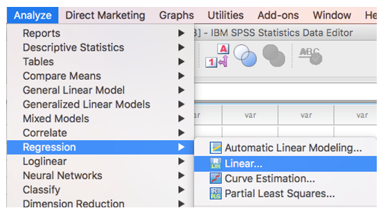 Step 2
We add Satisfaction with Life as our dependent variable and add Stress from Studying as our independent variable. Stress from Studying is our known predictor that is why it was added to our model first (Block 1). To add other two predictors, we must first click Next.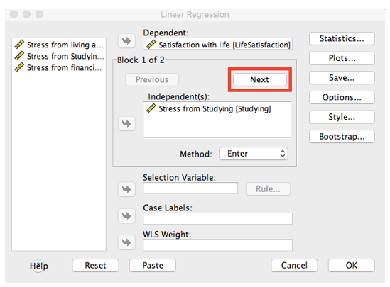 Step 3
By clicking Next, we enabled a second block. We add our two remaining predictors (Stress from Living away From Family and Stress from Financial Issues) into this separate block.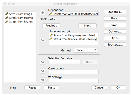 Step 4
We click on Statistics and tick the box R square change as we are interested in seeing if adding our two new predictors significantly improves our model. We click Continue and then Paste. We copy the command in Syntax and click Run.
Output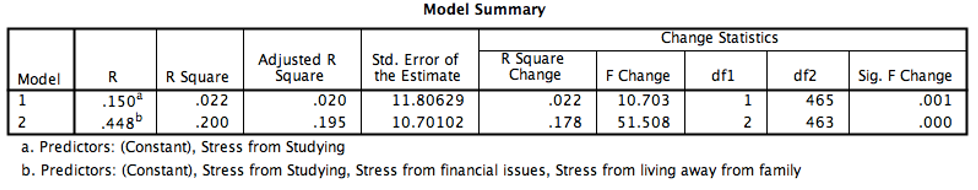 Model 1 that we entered first was the main predictor Stress from Studying. Then we have Model 2 where in addition to what we added in Model 1, Stress from Living Away from Family and Stress from Financial Issues were also added. We can see that Model 1 is significant and that the predictor significantly contributes to the outcome. However, by adding the two new predictors in the equation we can see that R Square Change in fact gets even larger, meaning that the added predictors in Model 2 explain the outcome above and beyond the predictor in Model 1 (Model 1: ∆R^2= .022, Model 2: ∆R^2= .178).
 When we look at different contributions of each predictor, we can see that after adding the two new predictors, the main predictor Stress from Studying is not a significant predictor anymore (p = .053). Thus, adding Stress from Living Away from Family and Stress from Financial Issues to the equation make our model a better predictor of the outcome, making Stress from Studying not a significant contributor to the outcome anymore.
Conclusion
Hierarchical multiple regression is a method of entering predictors into the regression model in a hierarchical order with known predictors added first and any new predictors we are interested in added after in separate blocks. We use it when we want to see the unique predictive influence of a new predictor on the outcome as all the known predictors are held constant.
By Petra Lipnik (University of Dundee, Academic Year 2016-17)
Hierarchical multiple regression is one of the methods of adding predictors into the multiple regression model where experimenter decides the order in which variables are entered into the model.
What Is A Multiple Regression?
Multiple regression is a natural extension of simple linear regression and is used when we want to predict outcome from multiple predictors. The general purpose of multiple regression is to learn more about the relationship between several independent variables or predictors and a dependent variable or an outcome. It is a hypothetical model of the relationship between several variables.
Adding PredictorsDoes the order in which we enter predictors matter?
In theory, it shouldn’t as the regression equation is of additive nature. In practice, however, all predictors correlate with each other to some extent and it is nearly impossible to find two predictors that are completely unrelated to each other. As soon as predictors are correlated there is a change in beta weight whenever a new predictor is added to the equation. Therefore, the answer is yes, the order does matter whenever the predictors are correlated.
Different methods of adding predictors to the regression model are:
- Forced entry, where all predictors are entered simultaneously.
- Stepwise, where predictors are selected using their semi-partial correlation with the outcome.
- Hierarchical, where the researcher decides the order in which variables are entered into the model.
In hierarchical multiple regression, we add the known predictors into the regression model first, with new predictors entered in separate blocks. The predictor is chosen to be added in the first block based on a theory or previous research that has shown that it is the main driving predictor to predict our outcome. The new predictors that we are interested in are then added in separate blocks. This way we can see the contribution of the new predictor when all other predictors are held constant.
When running hierarchical multiple regression we look at two things:
R^2 change, which tells us whether adding new predictors to our model improves our model significantly.
Beta weights of all our predictors, because we want to see how good our predictors are.
Remember! Hierarchical multiple regression relies on the researchers to know what they are doing as they make all the decisions.
When Would You Use It
We use hierarchical regression when we want to see whether predictors of our interest explain statistically significant amount of variance in our outcome after controlling for all other predictors. For example, we would use it when testing a new theory, as it tells us if in addition to this main predictor that we have, are there any other predictors that may contribute to the model above and beyond the one that is already there.
Example
Let’s assume that students studying abroad in UK filled out a questionnaire where they were asked to rate their Stress from Studying, Stress from Living Away from their Families, Stress from Financial Issues and their Satisfaction with Life. Let’s say that previous studies have shown that the Stress from Studying is the most important predictor for Life Satisfaction and we would like to know whether Stress from Living Away from Families and Stress from Financial Issues make an additional contribution to explaining Satisfaction with Life.
Step 1
Before running the analysis, we made sure that all the assumptions were met. To run a hierarchical multiple regression in SPSS we click Analyze --> Regression --> Linear.
Step 2We add Satisfaction with Life as our dependent variable and add Stress from Studying as our independent variable. Stress from Studying is our known predictor that is why it was added to our model first (Block 1). To add other two predictors, we must first click Next.
Step 3By clicking Next, we enabled a second block. We add our two remaining predictors (Stress from Living away From Family and Stress from Financial Issues) into this separate block.
Step 4We click on Statistics and tick the box R square change as we are interested in seeing if adding our two new predictors significantly improves our model.
We click Continue and then Paste. We copy the command in Syntax and click Run.Output
Model 1 that we entered first was the main predictor Stress from Studying. Then we have Model 2 where in addition to what we added in Model 1, Stress from Living Away from Family and Stress from Financial Issues were also added. We can see that Model 1 is significant and that the predictor significantly contributes to the outcome. However, by adding the two new predictors in the equation we can see that R Square Change in fact gets even larger, meaning that the added predictors in Model 2 explain the outcome above and beyond the predictor in Model 1 (Model 1: ∆R^2= .022, Model 2: ∆R^2= .178).
When we look at different contributions of each predictor, we can see that after adding the two new predictors, the main predictor Stress from Studying is not a significant predictor anymore (p = .053). Thus, adding Stress from Living Away from Family and Stress from Financial Issues to the equation make our model a better predictor of the outcome, making Stress from Studying not a significant contributor to the outcome anymore.Conclusion
Hierarchical multiple regression is a method of entering predictors into the regression model in a hierarchical order with known predictors added first and any new predictors we are interested in added after in separate blocks. We use it when we want to see the unique predictive influence of a new predictor on the outcome as all the known predictors are held constant.
By Petra Lipnik (University of Dundee, Academic Year 2016-17)
Overview
Multicollinearity is when two or more predictors, or independent variables, in a multiple linear regression are highly correlated to one another. This can create unreliable or misleading results and can make it difficult to determine the unique value of one variable in predicting an outcome.
What is multicollinearity?
Multicollinearity is a problem that can occur within a multiple regression model. A multiple linear regression allows us to predict an outcome based on the value of two or more independent variables. We would therefore expect there to be a correlation between the independent variable and the dependent variable, however multicollinearity exists when there are also strong correlations between the predictor variables. When multicollinearity occurs, it violates the assumption of no multicollinearity within the multiple regression and can cause a number of problems.
Example of multicollinearity
We may have a research question that aims to look at different predictors of self-esteem including BMI, income, social groups, and time spent at the gym. Two of these predictors might be Body Mass Index (BMI) and time spend at the gym, however they may have a high negative correlation to one another as BMI decreases as you spend more time at the gym.
Why is this a problem?
Determining the unique value of a predictor. Whilst the multiple regression model looks at the combined effect of all of the independent variables on the outcome, we may also be interested in learning about how each of these independent variables uniquely impacts the outcome, which can be hindered when multicollinearity is present in the data. This is because when two predictors share a large amount of variance it can be difficult to disentangle the effects each has on the outcome in order to determine which predictor has the biggest effect on the outcome.
Creating confusing or misleading results: Multicollinearity can adversely affect the regression estimates and significantly reduce the statistical power of the analysis. This is because multicollinearity increases the standard errors of the betas which decreases the likelihood that our sample is a true representation of population and can make the coefficient estimates difficult to interpret.
Indicators of multicollinearity
There are a number of indications that may suggest that there is multicollinearity in our data. One of these signals is that we may get a significant F value in the multiple regression, but the t-values that measure the unique contribution of predictors is non-significant. This may indicate that the variance accounted for in the outcome by a predictor is being controlled for by another predictor with which it is highly correlated. This may also be indicated by a dramatic change in the regression coefficients when a variable is added or removed from the equation. Additionally, having a different directionality than would be theoretically expected between the predictor and the outcome may indicate multicollinearity.
How to check for multicollinearity
Visually. One of the ways that we can check for multicollinearity in a multiple regression is through the use of a scatterplot matrix. This presents a visual representation which allows us to determine if there is a linear relationship between multiple variables and can alert us to possible cases of multicollinearity. For example, in the figure we can see that there is likely a relationship between BMI and time spent at the gym. Alternatively, you could use a scatterplot if you were investigating the relationship between two predictors. If the scatterplots suggested multicollinearity then we would also want to check these numerically.
Numerically. There are three numerical methods that we can use to determine if we have multicollinearity in our data. The first method is to check if our variables are highly correlated by looking at the Pearson correlations. We can see that BMI and time spent at the gym have a very strong negative correlation indicating that as time at the gym increases, BMI decreases, however this does not infer anything about causation.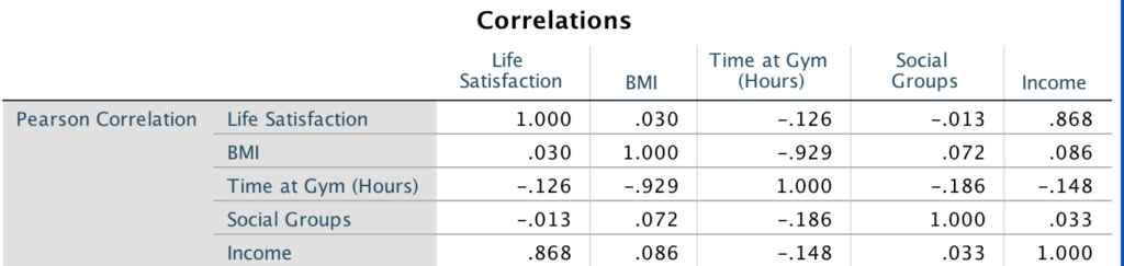 Whilst we can typically expect some correlation between variables, anything ± 0.8 is an indicator for multicollinearity.
We can also look the Variance Inflation Factor (VIF) which measures how much the standard errors and the variances of the correlation coefficients is inflated due to multicollinearity in the model. Additionally, the tolerance level tells us where a sampled population falls in a specified population. If the VIF is over 10, or if the Tolerance is lower than 0.2 then this may indicate the existence of multicollinearity. When we inspect the tolerance and VIF values then we can see that although the VIF is less than 10 for BMI and time spent at the gym this remains very high, and the tolerance levels are less than 0.2 indicating that the variables are highly correlated. The remainder of the predictors do not indicate cause for concern.
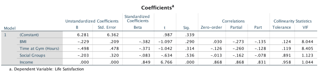 How to resolve the problem
There are a number of options to solve multicollinearity. One of the options may be to remove one of the variables that is highly correlated to another. This may be based upon prior theoretical or empirical knowledge or could be determined through a stepwise comparison. Another option may be to combine the two variables if they represent the same construct. For example, BMI and time spent at the gym may be collated to measure “self-image.”
By Emily Fairclough (University of Dundee, Academic Year 2017-18)
Multicollinearity is when two or more predictors, or independent variables, in a multiple linear regression are highly correlated to one another. This can create unreliable or misleading results and can make it difficult to determine the unique value of one variable in predicting an outcome.
What is multicollinearity?
Multicollinearity is a problem that can occur within a multiple regression model. A multiple linear regression allows us to predict an outcome based on the value of two or more independent variables. We would therefore expect there to be a correlation between the independent variable and the dependent variable, however multicollinearity exists when there are also strong correlations between the predictor variables. When multicollinearity occurs, it violates the assumption of no multicollinearity within the multiple regression and can cause a number of problems.
Example of multicollinearity
We may have a research question that aims to look at different predictors of self-esteem including BMI, income, social groups, and time spent at the gym. Two of these predictors might be Body Mass Index (BMI) and time spend at the gym, however they may have a high negative correlation to one another as BMI decreases as you spend more time at the gym.
Why is this a problem?
Determining the unique value of a predictor. Whilst the multiple regression model looks at the combined effect of all of the independent variables on the outcome, we may also be interested in learning about how each of these independent variables uniquely impacts the outcome, which can be hindered when multicollinearity is present in the data. This is because when two predictors share a large amount of variance it can be difficult to disentangle the effects each has on the outcome in order to determine which predictor has the biggest effect on the outcome.
Creating confusing or misleading results: Multicollinearity can adversely affect the regression estimates and significantly reduce the statistical power of the analysis. This is because multicollinearity increases the standard errors of the betas which decreases the likelihood that our sample is a true representation of population and can make the coefficient estimates difficult to interpret.
Indicators of multicollinearity
There are a number of indications that may suggest that there is multicollinearity in our data. One of these signals is that we may get a significant F value in the multiple regression, but the t-values that measure the unique contribution of predictors is non-significant. This may indicate that the variance accounted for in the outcome by a predictor is being controlled for by another predictor with which it is highly correlated. This may also be indicated by a dramatic change in the regression coefficients when a variable is added or removed from the equation. Additionally, having a different directionality than would be theoretically expected between the predictor and the outcome may indicate multicollinearity.
How to check for multicollinearity
Visually.
One of the ways that we can check for multicollinearity in a multiple regression is through the use of a scatterplot matrix. This presents a visual representation which allows us to determine if there is a linear relationship between multiple variables and can alert us to possible cases of multicollinearity. For example, in the figure we can see that there is likely a relationship between BMI and time spent at the gym. Alternatively, you could use a scatterplot if you were investigating the relationship between two predictors. If the scatterplots suggested multicollinearity then we would also want to check these numerically.Numerically. There are three numerical methods that we can use to determine if we have multicollinearity in our data. The first method is to check if our variables are highly correlated by looking at the Pearson correlations. We can see that BMI and time spent at the gym have a very strong negative correlation indicating that as time at the gym increases, BMI decreases, however this does not infer anything about causation.
Whilst we can typically expect some correlation between variables, anything ± 0.8 is an indicator for multicollinearity.We can also look the Variance Inflation Factor (VIF) which measures how much the standard errors and the variances of the correlation coefficients is inflated due to multicollinearity in the model. Additionally, the tolerance level tells us where a sampled population falls in a specified population. If the VIF is over 10, or if the Tolerance is lower than 0.2 then this may indicate the existence of multicollinearity. When we inspect the tolerance and VIF values then we can see that although the VIF is less than 10 for BMI and time spent at the gym this remains very high, and the tolerance levels are less than 0.2 indicating that the variables are highly correlated. The remainder of the predictors do not indicate cause for concern.
How to resolve the problemThere are a number of options to solve multicollinearity. One of the options may be to remove one of the variables that is highly correlated to another. This may be based upon prior theoretical or empirical knowledge or could be determined through a stepwise comparison. Another option may be to combine the two variables if they represent the same construct. For example, BMI and time spent at the gym may be collated to measure “self-image.”
By Emily Fairclough (University of Dundee, Academic Year 2017-18)
Dare to check your knowledge?
Take The Big Knowledge Test by D. Anderson
(University of Dundee, Academic Year 2015-16)